CDC (changed data capture)

The data warehouse stores the history of the data changes, so you need to sign in to submit only the changed data since the last update in DWH.

Goal:

• To be sure that the isolation of the changed data
• Provide certain type of change (insert, delete, update)
• Ensure batch downloading changes in DWH

Solution:

There are several ways to detect changes:

1. Analysis of the column audit or timestamp
The table is added to the system source column contains the date and time of insertion or last update. The value of the column is usually filled with triggers that run automatically when you insert or update. In some cases, in place of the time you can use a monotonically increasing numeric code audit.

cons:

• increasing the load on the database system resources and slowing down data modifications because of the trigger;
• if these columns are filled not trigger, then ensure the accuracy of change detection is not possible;
• it is impossible to determine whether the removal;
• problems with the time change to the source server or not synchronized with time DWH (for timestamp);
• storage of digital codes of the last audit exemption for each table (for digital labels).

2. Analysis of tables with the change log

For each tracked table to create a log table that stores all the line after modification, the modification time, and type of modification. Filling a table is done via a trigger to insert, delete, and update the tracked table.

cons:

• increasing the load on the database system resources and slowing down data modifications because of the trigger;
• need to be able to aggregate changes in one line. Since the magazine provides all the changes, the hour might happen inserting rows, updating and subsequent removal;
• the need for periodic cleaning of the magazines;
• problems with the time change to the source server or not synchronized with time DWH;

3. Analysis of log files

The method is to periodically copy the redo log (redo log) database and analysis of these logs in order to highlight the transaction affecting the table you are interested in.

cons:

• magazines not supported by all DBMS;
• need to be able to aggregate changes in one line;
• loss of information about changes in the case of carrying out administrative work.

Often crowded logs that blocks further transactions. When this happens in a commercial transaction system, the reaction responsible DBA is to clean the logs. If you have sorted out all the options, and log analysis was the only appropriate, it is necessary to convince the DBA to create for you a special transaction log.

4. Full comparison

At full comparison holds the full picture of the table on the last day, and compared to each entry with today's version of the search for each change. Gives a guaranteed change detection.

cons:

• the cost of the disk subsystem;
• cost comparison;
• implementation of the algorithm for calculating checksums.

ETL Team Mission

The main mission of the ETL team is to build the DWH.
More deeply, the ETL team have to develop ETL framework which can effectively:

• Deliver data most effectively to end user tools;
• Add value to data in the cleaning and conforming steps;
• Protect and document the lineage of data.

The ETL framework have to cover the following main points:

• Extracting data from the sources;
• Keep an eye on quality of data and cleaning data;
• Conforming the labels and measures in the data to achieve consistency across the sources;
• Delivering data in a business layer, where it can be accessed by BI tools and business users.

In addition, I want to mention about responsibility of ETL guys, they are responsible for the quality and accuracy of data and they do not hesitate to contact business in case of technical problems or in case of unclear business requirements.

We, technical staff, all work for our business departments and help to make right and accuracy business decision, that's why we have to work in collaboration with business, although we are technical guys and used to work with machines.

Data Models in DWH

The data model is a corporate repository ER-model (Entity-relationship model - the model "entity-relationship"), described on several levels set of interconnected entities, which are grouped by functional area and reflect the needs of the business in the analytical analysis and reporting.

General corporate data model repository is developed consistently and consists of:

• conceptual data model;
• logical data model;
• physical data model.

Conceptual Model

Conceptual model of a data warehouse is a description of the main (basic) entities and relations between them. The conceptual model is a reflection of the subject areas in which it is planned to build a data warehouse.

Logic model

Logical model extends the conceptual definitions for entities by their attributes, descriptions and restrictions, clarifies the composition of entities and relationships between them.

Physical model

Physical data model describes the implementation of a logical model of objects at the level of a specific database objects.

Comparison of models of different levels

The table below presents a comparative analysis of models of different levels.

Using bitmap indexes in databases

Kelly Sommers posted a great article on the internals of bitmap indexes:

"There are many different data structures used in databases to create indexes used to quickly evaluate queries. Each one has different strengths and weaknesses based on the tradeoffs they make on memory, cpu and storage (if persisted). One of these types of indexes is called a bitmap index. For the purpose of this post I’m going to be using relational database terminology but the same techniques can apply to different database types like column oriented databases or many others non-relational databases.

A bitmap index represents membership. A bitmap index is an array of bits, a bit represents each row where each bit set to 1 represents membership in the set.

To illustrate this better lets create an example table with 4 rows but consider it could be a table with 100 million rows.

TABLE USERS

UserId	Name	Country
100	Jane	Canada
101	Joe	USA
102	John	Germany
103	Julie	USA

Creating a bitmap index on the country column would give us 3 bitmap indexes (3 arrays of bits) that looks like the following.

COUNTRY INDEX

Canada	[1, 0, 0, 0]
USA	[0, 1, 0, 1]
Germany	[0, 0, 1, 0]

Now a bitmap index for the Name column which creates 4 bitmap indexes.

NAME INDEX

Jane	[1, 0, 0, 0]
Joe	[0, 1, 0, 0]
John	[0, 0, 1, 0]
Julie	[0, 0, 0, 1]

In addition to the bitmap indexes, we need a map that maps index positions to rows in the database (more on why later).

ROW MAP

[100, 101, 102, 103]

Types of data

Bitmap indexes do well at indexing categorial data with well defined values like countries, dates and ages as a few examples. Bitmap indexes don’t do well with numerical data with continuous values like prices or kilometres per hour that you may want to sum or average. A 1 in the array of bits represents membership in the set for a unique term which makes them suitable for WHERE A = B type evaluations and not WHERE A > B evaluations.

Memory and storage

If you have 100 million rows in your database, the storage for the Country column index would be 3 bitmap indexes with 100 million bits (12 megabytes) each taking a total 36MB.

Using bitmap indexes means managing a lot of indexes because you need a new array of bits per unique term. That’s one of the cons of a bitmap index. If you have 100 million rows and each has a unique term (say a timestamp) you would create bitmap indexes for each timestamp where only 1 bit is set out of 100 million bits.

Fortunately there are ways to tackle this problem called Compressed Bitmaps which I will cover later.

Evaluating a query

With the indexes and row map defined we can jump back to the high level and explain how a query like this works.

SELECT *FROM USERS
WHERE Name = ‘Julie’ AND Country = ‘USA’

There’s a lot of material and research on how to optimize query operations such as choosing which order to do things based on cardinality and many other aspects. In these examples I’m not explaining the process of optimizing a query execution plan, just explaining the basics.

To evaluate which rows match the criteria we can do bitwise operations like bitwise AND and OR’s.

STEP 1: Evaluate Name = ‘Julie’ AND Country = ‘USA’

We take the 2 bitmap indexes that represent the terms “Julie” and “USA” and we bitwise AND them.

    0001 (Julie)
AND 0101 (USA)
  = 0001

STEP 2: Map results to row map

Take all the set bits and map the row key.

[0, 0, 0, 1]
= rowmap[3]
= rows["103"]

STEP 3: Select results

With the results from the where clause evaluated into row keys now we can use however our database storage works to fetch the rows and the columns selected in the query to return.

Deletes

Depending on the database implementation, deleting a row in a database may cause a bunch of index rebuilds to occur but luckily with bitmap indexes you can still respond to queries with responses that exclude the deleted rows of data while these indexes rebuild in the background. Create a new bitmap index that represents deleted rows then bitwise AND against this bitmap index with any query results. In a bitmap index that represents deletes, a bit set to 1 represents a valid row and a bit set to 0 represents a deleted row.

Using the query mentioned above, if we deleted Julie the operations would look something like this.

    0001 (Julie)
AND 0101 (USA)
AND 1110 (Deletes)
  = 0000 (No matching rows!)

The bitmap index representing deletes is temporary and can be removed once the indexes affected by the row deletion have been rebuilt.

Group By and Joins

Bitmap indexes can be used for evaluating a lot of different parts of a query such as GROUP BY and JOIN clauses. Evaluating a join is a multi-step process because you need to evaluate the bitmap indexes from the right side join table and then take the resulting bitmap and bitwise AND it against the query result on the left side like we did on the deletes example. One to many to one relationships get even more complicated because there is an intermediary table facilitating the relationship. Explaining joins is a much more involved example I will leave for another blog post.

Bitmap indexes in OLAP databases

An OLAP (online analytical processing) database is typically used for reporting and business intelligence where there is a need to query data in many different ways (dimensions) with quick response times and is sometimes called an “OLAP Cube”. OLAP data is usually stored with a star schema where there is a fact table and multiple dimension tables. If we were analyzing sales, the sales table would be the fact table. Country and day of week would be dimension tables. This star schema would allow us to do analytical queries answering questions like “top 10 sales by country on Saturday” giving you insight on which countries you may want to increase promotions.

Some OLAP databases use bitmap indexes. When the OLAP cube is being generated it creates pre-calculated results so that queries can be extremely fast. When the cube is being generated it’s going through a materialization stage where it is evaluating every possible bitmap index combination for the dimension tables and creates all the resulting bitmaps.

The nice thing about using bitmap indexes in an OLAP database, since everything is an array of bits, you can choose not to materialize everything. If a pre-calculated result explodes the cube due to the size of possible combinations you can do what is called partial materialization where you don’t materialize everything but you can still evaluate bitmaps from parts that are materialized with bitmaps that aren’t materialized.

Accelerating with SIMD & GPU’s

Included in many modern processors is SSE2 which provides SIMD (Single instruction, multiple data). Using SIMD to evaluate the bitwise AND or bitwise OR operations would give the ability to evaluate (depending on CPU) 128 bits at once. With Intel AVX (Advanced Vector Extensions) in Sandy Bridge and AMD BullDozer up to 256 bits is supported. This would be a significant increase in performance for the operations explained earlier.

Using GPGPU could also accelerate processing even further but this poses additional challenges around getting data in and out of the GPU VRAM. If your indexes are larger than the VRAM available you will need to swap data in and out of the GPU many times.

Compressed Bitmap Index

One of the cons to using bitmap indexes is the amount of bitmap indexes that get created. You need to create one bitmap index the size of the row count per unique term. Luckily run-length encoding fits this problem really well. If you have really high cardinality columns, you will likely have most bits set to 0 and these can be compressed very well. Compressed bitmaps allow you to do the bitwise AND and bitwise OR operations in the compressed form avoiding having to decompress these large bitmaps before using them. Sparsity of membership when using run-length encoding will dictate how effective the compression rate is.

You can find some really good compressed bitmap implementations at the following links.

C#
Java
C++
Ruby

Conclusion

Compressed bitmap indexes can be really useful for evaluating queries on really large datasets quickly and offer a good compromise between memory efficiency and processing speed since in many cases they can be faster than uncompressed bitmaps. I only cover some basic uses of bitmap indexes, there are a lot of different ways to approach data indexing and query execution plans."

ETL Tool versus Hand Coding

If you are planning DWH project, You should consider ETL Tool.
I found very interesting and useful article of Gary Nissen where he compared two various approaches.

ETL Tool vs Scripting.

Advantages of tool-based ETL

1. Simpler, faster, cheaper development. The ETL tool cost will make up for itself in projects that are large enough or sophisticated enough.
2. Many ETL tools have integrated metadata repositories that can synchronize metadata from source systems, target databases and other BI tools.
3. Most ETL tools enforce a consistent metadata driven methodology that all developers must follow.
4. Data flow and data lineage documentation can often be automatically generated from a metadata repository.
5. ETL tools have connectors pre-built for many source and target systems. So, if you are working with many sources or targets, you will find many advantages in a tool-based approach.
6. Most ETL tools deliver good performance even for very large data sets. If your ETL data volume is really large, or it will be large in a year or two, you should seriously consider a tool-based option.
7. Some ETL tools help you conduct change impact analysis further down the road.

 Advantages of hand-coded ETL

1. Automated unit testing tools are available in a hand-coded system, but not with a tool-based approach. For example, the JUnit library (http://junit.org) is a highly regarded and well-supported tool for unit testing Java programs. There are also similar packages for other languages. Another common approach to unit testing is to use a scripting language, like TCL or Python, to setup test data, run an ETL process and verify the results. Automating the testing process through one of these methods will significantly improve the productivity of your QA staff and the quality of your deliverables.
2. Object-oriented programming techniques help you to make all of your transformations consistent for error reporting, validation, and metadata updates. You may not have this degree of control with the parameter setting and snippet programming style of ETL tools.
3. Metadata can be more directly managed by hand-coded systems. Actually, metadata driven hand-coded systems are much more flexible than any alternative.
4. A brief requirements analysis of an ETL system quickly points you towards file-based processing, not database stored procedures. File-based processes are more direct. They are simply coded, easily tested and well understood.
5. A tool-based approach will limit you to the tool vendor’s abilities and their unique scripting language. But, a hand-coded system can be developed in a common and well-known language. In fairness, all the ETL tools allow “escapes” to standard programming languages in isolated modules.
6. Hand-coded ETL provides unlimited flexibility, if that is indeed what you need. You can literally do anything you want. There are many instances where a unique approach or a different language can provide a big advantage.

In addition, be aware about you IT guys, who used to change job sometimes, and it is a fact, that hand-code of good programmer very often is impossible to understand. Moreover, hand code is quite difficult to scale.

Columnar DBMS - principle, advantages and scope

The middle of the 2000s was marked by rapid growth of columnar DBMS. Vertica, ParAccel, Kognito, Infobright, SAND and others joined the club columnar DBMS and diluted proud solitude Sybase IQ, founded it in the early 90s. In this article I will discover the reasons for the popularity of the idea in a column of data storage, operation and use of the area columnar DBMS.

Let's start with the fact that popular nowadays relational databases - Oracle, SQL Server, MySQL, DB2, Postgresql and etc. Based on the architecture, its history is counted more since 1970s, when transistor radios were sideburns long, flared trousers, a database in the world dominated by hierarchical and network data management system. The main task of the database, then, is to support beginning in the 1960s, a massive shift from paper records of economic activity to the computer. A wealth of information from paper documents was transferred to a database accounting systems that were supposed to securely store all incoming information and, if necessary, to quickly find them. These requirements led to the architectural features of relational databases, the remaining hitherto virtually unchanged: progressive storage, indexing records and logging operations.

Under the interline storage is usually understood the physical storage of all rows in the table in the form of a record in which the fields are sequentially one after the other, and the last field recordings, in general, is the first next record. Something like this:

[A1, B1, C1], [A2, B2, C2], [A3, B3, C3] ...

where A, B and C - a field (columns), and 1.2 and 3 - record number (row).

Such storage is extremely convenient for frequent operations to add new rows in the database, usually stored on a hard drive - in fact in this case, a new record can be added entirely in just one pass of the drive heads. Significant speed restrictions imposed by the HD, caused the need to conduct specific indexes, which would allow to find the desired item on the disc in the minimum number of passes head HDD. Typically, several indices formed, depending on which fields required to make the search, which increases the volume of the database on a disk is sometimes several times. For resiliency traditional DBMS automatically duplicate transactions in the log, which leads to even more space occupied on disk. As a result, for example, an Oracle database average takes up 5 times more space than the volume of payload data therein. For srednepotolochnoy database to DB2, this ratio is even more - 7: 1.

However, in the 1990s, the spread of information systems analysis and storage of data used for the analysis of management accounting systems in the accumulated data, it became clear that the nature of the load in these two types of systems is radically different.

If transactional applications characterized by very frequent small transactions add or change one or more records (insert / update), in the case of analytical systems opposite picture - the largest load is created relatively rare but serious samples (select) the hundreds of thousands and millions of records, often with groups and calculation of totals (so-called units). Write operations wherein a low, often less than 1% of the total. And often you record large blocks (bulk load). It should be noted that the analytical sample is one important feature - they usually contain only a few fields. On average, in the analytic SQL-user request them rarely more than 7-8. This is due to the fact that the human mind is unable to properly absorb information more than 5-7 sections.

However, what happens if you choose, for example, only 3 fields from the table, in which there are only 50? Due to progressive data storage in traditional DBMS (required, as we remember, for frequent operations to add new entries to the accounting systems) will be read completely all lines completely with all fields. This means that no matter whether we need only 50 fields or 3, with the disc in any case they are read entirely, passed through the disk controller, input and output to the processor, which has only necessary to take away request. Unfortunately, the channels of disk IO are usually the main limiter performance analytical systems. As a result, the effectiveness of traditional RDBMS in the performance of this query can be reduced by 10-15 times because of the imminent reading unnecessary data. And Moore's Law on the rate of input-output disk drives much weaker than the speed of processors and amount of memory. So, apparently, the situation will only get worse.

To solve this problem are called columnar DBMS. The basic idea of columnar database - it can store data in rows, as do traditional DBMS, and on columns. This means that from the point of view of SQL-client data is typically represented as a table, but a table is physically these plurality of columns, each of which is essentially a table of one field. At the same physical disk space value of one field are stored one after the other - something like this:

[A1, A2, A3], [B1, B2, B3], [C1, C2, C3], etc.

This data organization leads to the fact that when the select which featured only three fields of 50 fields in the table, the disc will be physically read only 3 columns. This means that the load on the input-output channel will be about 50/3 = 17 times smaller than if the same in traditional database query.

In addition, when columnar data storage appears a great opportunity to greatly compress the data as a single column of the table data is generally of the same type can not be said about the line. Compression algorithms may be different. Here is an example of one of them - the so-called Run-Length Encoding (RLE):

If we have a table with 100 million records, made within one year, in the column "Date" will actually be stored for no more than 366 possible values, as of the year no more than 366 days (including leap years). So we can 100 million sorted values in this field is replaced by 366 pairs of values of the form <date, the number of times> and store them on disk in this form. Thus they will occupy approximately 100 thousand. Times less space, which also contributes to the query performance.

From a developer's perspective, columnar DBMS usually correspond ACID and support largely SQL-99 standard.

Resume

Columnar DBMS designed to solve the problem of inefficiency of traditional databases in analytical systems and systems in the vast majority of operations such as 'read'. They allow for cheaper and less powerful hardware to get a speed boost query performance at 5, 10 and sometimes even 100 times, while, thanks to compression, the data on the disk will take 5-10 times less than in the case of traditional DBMS.

In columnar DBMS there are disadvantages - they are slow to write, not suitable for transactional systems, and as a rule, because of the "youth" have a number of limitations to the developer who is used to the development of traditional DBMS.

Columnar DBMS usually used in analytical systems class business intelligence (ROLAP) and analytical data warehouse (data warehouses). And the amount of data can be quite large - there are examples on 300-500TB and even cases with> 1PB of data.

Tableau Software + Cloudera Hadoop

Nowadays we have to work with really big volume of data. Unfortunately classical relation database are weak and can't handle this challenge. Of course, if we have 1 Mln $ we can buy MPP database such as Teradata, Vertica, Exadata or Netezza. But most organization starting look at Hadoop, especially on commercial distributives such as Apache or Cloudera.

It is not a secret that it is not easy to work with Hadoop, and you have to hire expensive geeks, who can work with this staff.

Anyway, lets imagine, that we have Cluster of Hadoop, in my case it is Cloudera Hadoop. And we, as BI professionals, need to do analytics on top of Hadoop, but unfortunately, we don't know Java in order to write MapReduce Jobs, and we start to look at Hive or Impala in order to work with usual SQL, of course with restrictions.

The Apache Hive ™ data warehouse software facilitates querying and managing large datasets residing in distributed storage. Hive provides a mechanism to project structure onto this data and query the data using a SQL-like language called HiveQL. At the same time this language also allows traditional map/reduce programmers to plug in their custom mappers and reducers when it is inconvenient or inefficient to express this logic in HiveQL.


Impala is a fully integrated, state-of-the-art analytic database architected specifically to leverage the flexibility and scalability strengths of Hadoop - combining the familiar SQL support and multi-user performance of a traditional analytic database with the rock-solid foundation of open source Apache Hadoop and the production-grade security and management extensions of Cloudera Enterprise.


But just SQL isn't enough for powerful analytics, we want Charts, drag and drop, slice and dice:)

Specially for us, leading BI platforms such as Tableau, Microstrategy, Pentaho and other make possible to connect Hadoop via Hive/Impala ODBC driver.

In my case I will demonstrate how you can establish connection between Hadoop and Tableau.

Let's start.

Get data
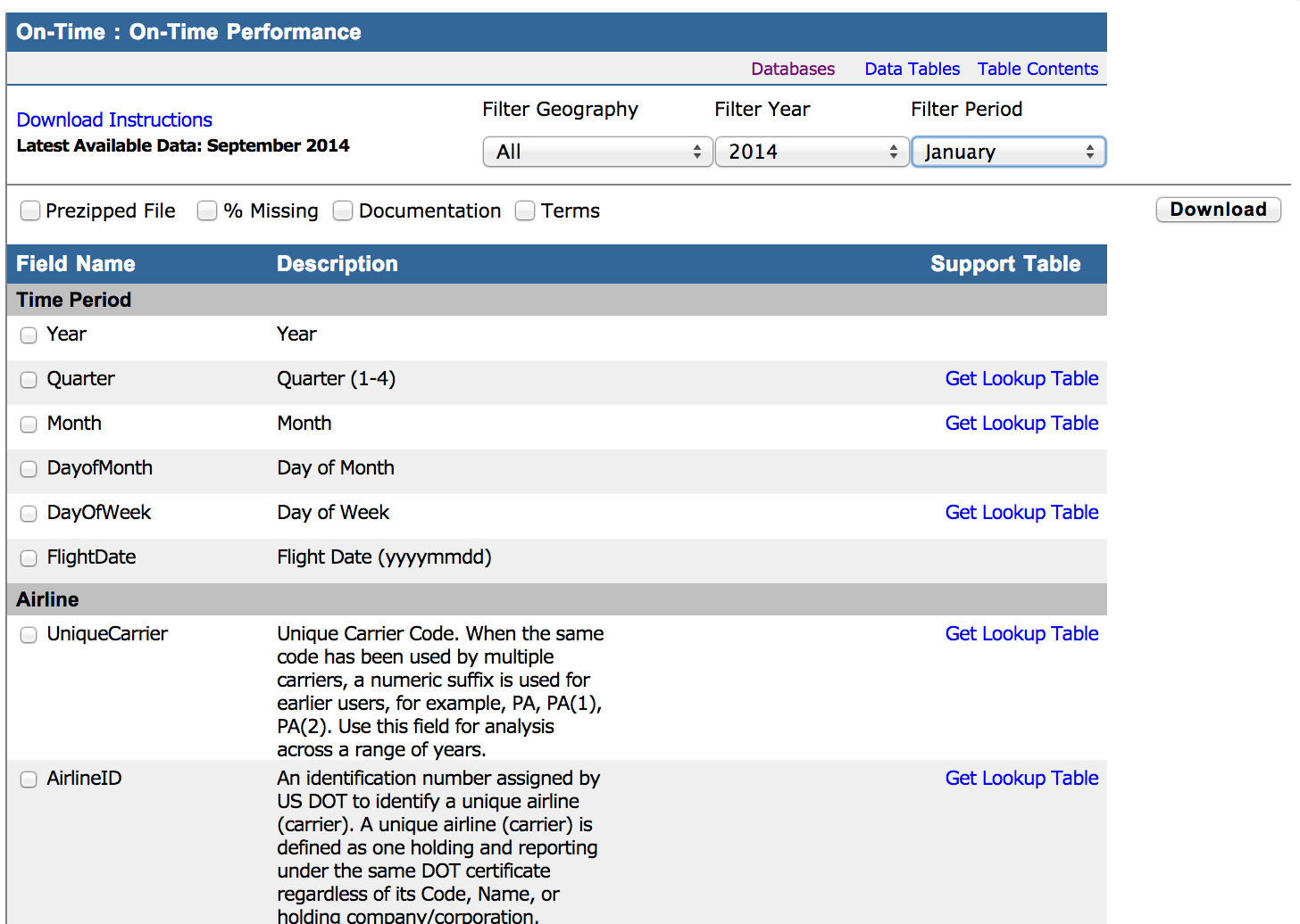
First of all, we need data. The best sample data and the most popular data in the Internet is Flight data.

The Bureau of Transportation Statistics has a web site dedicated to TranStats, which is the Intermodal Transportation Database. This database contains information that is regularly updated on aviation, maritime, highway, rail, and other modes of transportation. As described earlier, we will focus only on the Airline On-Time Performance data, which is
made available as a simple table that contains departure and arrival data for all the scheduled nonstop flights that occur exclusively within the United States of America. The data is reported on a monthly basis by U.S. certified carriers that account for at least one percent of the domestic scheduled passenger revenues. The flight data and a description

are available at the following URL: http://www.transtats.bts.gov/

In the left bar find Data Finder->By Mode->Aviation

Selecting the Aviation link will take you to a page that presents a list of aviation related databases. On this list, select the Airline On-Time Performance Data by clicking on the name of the database. This will take you to the next page, which shows more detailed information about the database we are interested in. Here you will click on the download link as shown in Figure:

Here you can download data for the specific month in CSV format:

But it is a long road to download all data since 1989:)

You can use command wget or curl and download all files via shell script. There is an example on my mac:

wget "http://www.transtats.bts.gov/Download/On_Time_Performance_1986_11.zip"

PS 11/86 - my birth year month:)

Small tip: you can use parameters and for in order to cut the road.

Finally,  we get data. 

Upload data

Now we have to upload data into Hadoop. 

I use HUE. 

Hue is a set of web applications that enable you to interact with a CDH cluster. Hue applications let you browse HDFS, manage a Hive metastore, and run Hive and Cloudera Impala queries, HBase and Sqoop commands, Pig scripts, MapReduce jobs, and Oozie workflows.

Hue Architecture

Hue applications run in a Web browser and require no client installation. 

The following figure illustrates how Hue works. Hue Server is a "container" web application that sits in between CDH and the browser. It hosts all the Hue web applications and communicates with CDH components.

Connect to HUE and go to file browser:

Push "Upload" and select or CSV file. 

Create database

Now we can create database "danoshin" via Metastore Manager:

Create table

We can create new table "flight" via Hive in our database

(with ~ I cut some fields, but you need all fields):

Parameters:

ROW FORMAT DELIMITED FIELDS TERMINATED BY ','  - specify delimiter;

LINES TERMINATED BY '\n' - end of row;

STORED AS TEXTFILE - type of file;

LOCATION '/user/danoshin/input/' - location in HDFS;

In case if file has header, we need delete it, you can do it Hive query: 

INSERT OVERWRITE TABLE FLIGHT

SELECT * FROM FLIGHT WHERE YEAR <> '"Year"'

Get data via Tableau
Now we can open Tableau and choose connection to Cloudera hive.
By default it has port 10000, be aware, you need to check, that service for connection to hadoop has to work.

If you are wondered about Hive and Hive2, there are some points for you:

• HiveServer2 Thrift API spec
• JDBC/ODBC HiveServer2 drivers
• Concurrent Thrift clients with memory leak fixes and session/config info
• Kerberos authentication
• Authorization to improve GRANT/ROLE and code injection vectors

When you type credentials, you can find your database and table:

Finally, you are almost there, just push "Go to worksheet"

There is small chart, and we can figure out, that WN airlines the most popular in that time:)

In addition, you can monitoring job execution in Job Manager:

Business Analytics - Paradigm Change

Business Analytics Paradigm Change from Dmitry Anoshin

Splunk 6.2 New Features

Splunk TRANSACTION Command

Splunk definition of the command:

Given events as input, this command finds transactions based on events that meet various constraints. Transactions are made up of the raw text (the _raw field) of each member, the time and date fields of the earliest member, as well as the union of all other fields of each member.

Additionally, the transaction command produces two fields to the raw events, duration and eventcount. The duration value is the difference between the timestamps for the first and last events in the transaction. The eventcount value is the number of events in the transaction.

• A transaction is any group of related events that span time

• Events can come from multiple applications or hosts

- Events related to a single purchase from an online store can span across an

application server, database, and e-commerce engine

- One email message can create multiple events as it travels through various queues

– Each event in the network traffic logs represents a single user generating a single http request

– Visiting a single website normally generates multiple http requests - HTML, JavaScript, CSS files

- Flash, Images, etc. 

• <field-list>

–  One field or a list of field names

–  The events are grouped into transactions based on the values of this field list

–  If a quoted list of fields is specified, events are grouped together if they have the same value for each of the fields

• Common constraints:

– <maxspan> | <maxpause> | <maxevents> | <startswith> | <endswith> | <keepevicted> 

• Here you can see a number of events that share the same JSESSIONID

• However, it is difficult to display or gain insight to what is happening

Example 1

Display customer transactions in the online store during the last 15 minutes.

• Use the transaction command to create a single event from a group of events that share the same value in a given field

• Transactions can cross multiple tiers (i.e., web server, application server) using a common field(s), in this example, JSESSIONID



Type in search:
sourcetype=access_combined | transaction JSESSIONID

Example 2
Display a table of what customers are doing in the online store during the last 60 minutes.
With the transaction command, you can also use tables to easily view the information that you want
Scenario ?

Type in search:
sourcetype=access_combined | transaction JSESSIONID | table JSESSIONID, action, product_name

Specific Fields of transaction:

• The transaction command produces some additional fields, such as:

–  duration – the difference between the timestamps for the first and last event in the transaction

–  eventcount – the number of events in the transaction

Example 3

Use of maxspan/maxpause

Display customer actions on the website during the last 4 hours.

• You can also define a max overall time span and max gap between events

Scenario ?

- maxspan=10m

         ▸ Maximum total time between the earliest and latest events

         ▸ If not specified, default is -1 (or no limit)

 - maxpause=1m

         ▸ Maximum total time between events 

         ▸ If not specified, default is -1 (or no limit)

Note

Assumptions: Transactions spanning more than 10 minutes with the same client IP are considered unrelated, nor can there be more than one 1 minute between any two related events.

Type in search:

sourcetype=access_combined | transaction clientip maxspan=10m maxpause=1m | eval duration = round(duration/60,2) | sort -duration | table clientip duration action | rename duration as "Time Spent", clientip as "Client IP",   action as "Client Actions"

Type in search:

sourcetype=access_combined | transaction clientip maxspan=10m maxpause=1m | eval duration = round(duration/60,2) | sort -duration | table clientip duration action | rename duration as "Time Spent", clientip as "Client IP",   action as "Client Actions"

Example 4

Use of startswith/endswith

Determine the length of time spent by customers in the online store to purchase.

• To form transactions based on terms, field values, or evaluations, use startswith and endswith options

• In this example, the first event in the transaction includes addtocart and the last event includes purchase

Type in search:

sourcetype=access_combined | transaction clientip startswith=action="addtocart" endswith=action="purchase" | table clientip,  JSESSIONID, product_name, action, duration, eventcount, price

Example 5

Investigating with Transactions

Find emails that were rejected during the last 24 hours.

• Transactions can be useful when a single event does not provide enough information

• This example searches email logs for the term “REJECT”

• Events that include the term don’t provide much information about the rejection Scenario ?



Type in search:

sourcetype=cisco_esa REJECT

Find emails that were rejected.

• By creating a transaction, we can then search and see additional events related to the rejection, such as:

- IP address of sender

- Reverse DNS lookup results

- Action taken by the mail system following the rejection

• mid – Message ID

• dcid – Delivery Connection ID 

• icid – Incoming Connection ID

Type in search:

sourcetype=cisco_esa | transaction mid dcid icid | search REJECT

Reporting on Transactions

• You can use statistics and reporting commands with transactions

• This example takes advantage of the duration field

–  It shows a trend of the mail queue slowing, then correcting, then slowing again

- Adding events to the transaction from additional hosts or sources can uncover the cause of the slowdown

Type in search:

sourcetype=cisco_esa | transaction mid dcid ion) | timechart avg(duration)

Transaction vs. Stats

• Use transaction when you

     –  Need to see events correlated together

     –  Must define event grouping based on start/end values

• Use stats when you:

     –  Want to see the results of a calculation

     –  Can group events based on a field value (e.g. "by src")

• When you have a choice, always use stats

     –  stats is faster and more efficient, especially in large Splunk environments

Lets consider example:

sourcetype=sales_entries                                                             sourcetype=sales_entries

| transaction CustomerID                                                             | stats count as eventcount

| table CustomerID eventcount                                                    by CustomerID        

Returned 101 by scanning 31,767 events                                    Returned 101 results by scanning                                

 in 0.802 seconds                                                                          31,797 events   in 0.499 seconds

  

    

Splunk Overview Presentation

What is Splunk?

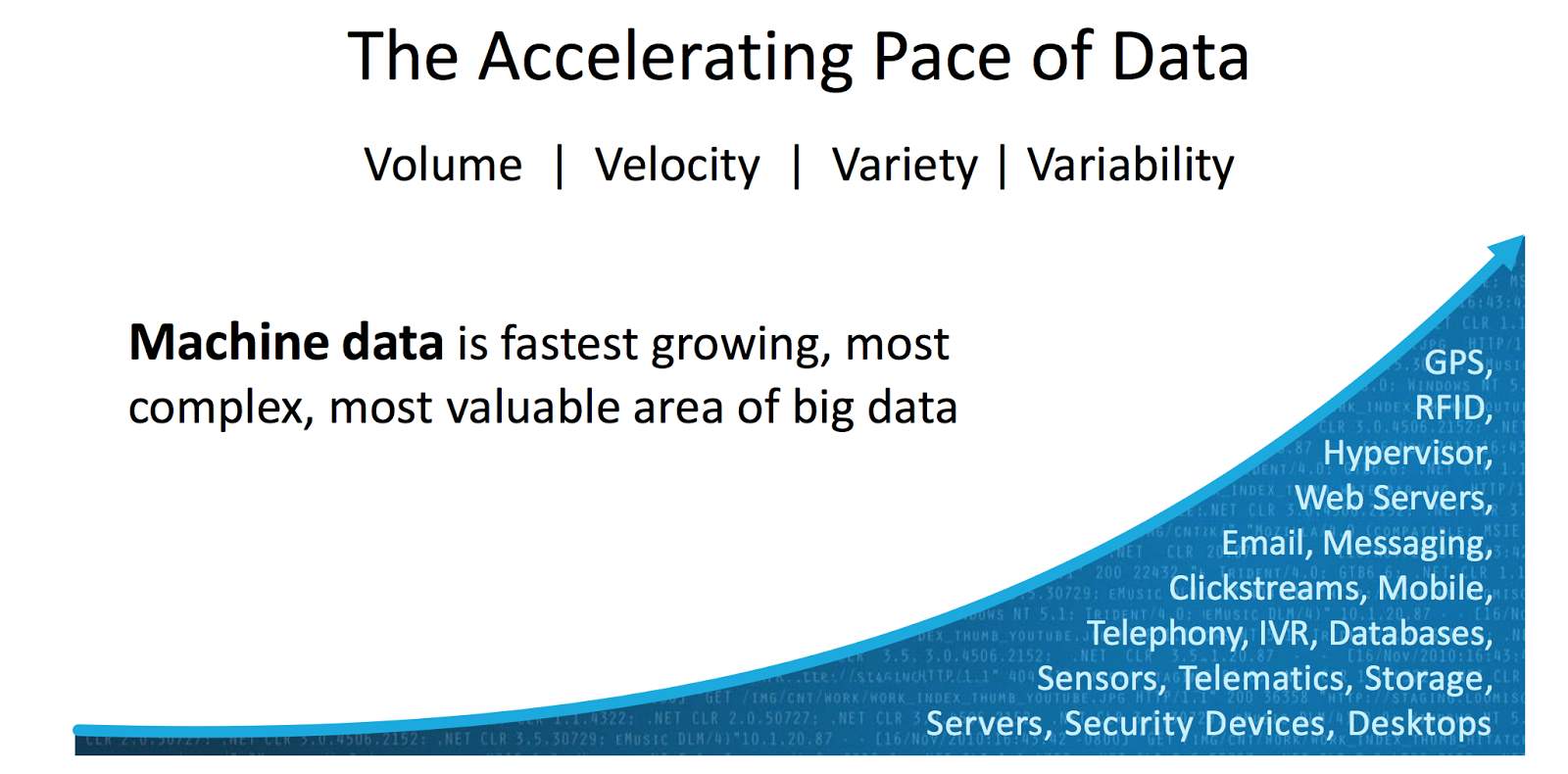
Technically speaking, Splunk is a time-series indexer, but to simplify things we will just say that it is a product that takes care of the three Vs very well. 

If we go to technical details, Splunk is key-value store, where key is a timestmap. In addition, it use MapReduce in order to process data.

Whereas most of the products that we described earlier had their origins in processing human-generated digital footprints, Splunk started as a product designed to process machine data. Because of these humble beginnings, Splunk is not always considered a player in big data. But that should not prevent you from using it to analyze big data belonging in the digital footprint category, because, as this book shows, Splunk does a great job of it. Splunk has three main functionalities: 

• Data collection, which can be done for static data or by monitoring changes and additions to files or complete directories on a real time basis. Data can also be collected from network ports or directly from programs or scripts. Additionally, Splunk can connect with relational databases to collect, insert or update data.
• Data indexing, in which the collected data is broken down into events, roughly equivalent to database records, or simply lines of data. Then the data is processed and a high performance index is updated, which points to the stored data.\
• Search and analysis. Using the Splunk Processing Language, you are able to search for data and manipulate it to obtain the desired results, whether in the form of reports or alerts. The results can be presented as individual events, tables, or charts.

Each one of these functionalities can scale independently; for example, the data collection component can scale to handle hundreds of thousands of servers. The data indexing functionality can scale to a large number of servers, which can be configured as distributed peers, and, if necessary, with a high availability option to transparently handle fault tolerance. The search heads, as the servers dedicated to the search and analysis functionality are known, can also scale to as many as needed. Additionally, each of these functionalities can be arranged in such a way that they can be optimized to accommodate geographical locations, time zones, data centers, or any other requirements. Splunk is so flexible regarding scalability that you can start with a single instance of the product running on your laptop and grow from there.

You can interact with Splunk by using SplunkWeb, the browser-based user interface, or directly using the command line interface (CLI). Splunk is flexible in that it can run on Windows or just about any variation of Unix.

Splunk is also a platform that can be used to develop applications to handle big data analytics. It has a powerful set of APIs that can be used with Python, Java, JavaScript, Ruby, PHP, and C#. The development of apps on top of Splunk is beyond the scope of this book; however, we do describe how to use some of the popular apps that are freely available. We will leave it at that, as all the rest of the book is about Splunk. 

What is BigData?

I found amazing definition of BigData in the book: BigData Analytics. Here is:


Big data is, admittedly, an overhyped buzzword used by software and hardware companies to boost their sales. Behind the hype, however, there is a real and extremely important technology trend with impressive business potential. Although big data is often associated with social media, we will show that it is about much more than that. Before we venture into definitions, however, let’s have a look at some facts about big data.
Back in 2001, Doug Laney from Meta Group (an IT research company acquired by Gartner in 2005) wrote
a research paper in which he stated that e-commerce had exploded data management along three dimensions: volumes, velocity, and variety. These are called the three Vs of big data and, as you would expect, a number of vendors have added more Vs to their own definitions.
Volume is the first thought that comes with big data: the big part. Some experts consider Petabytes the starting point of big data. As we generate more and more data, we are sure this starting point will keep growing. However, volume in itself is not a perfect criterion of big data, as we feel that the other two Vs have a more direct impact.
Velocity refers to the speed at which the data is being generated or the frequency with which it is delivered. Think of the stream of data coming from the sensors in the highways in the Los Angeles area, or the video cameras in some airports that scan and process faces in a crowd. There is also the click stream data of popular e-commerce web sites.
Variety is about all the different data and file types that are available. Just think about the music files in the iTunes store (about 28 million songs and over 30 billion downloads), or the movies in Netflix (over 75,000), the articles in
the New York Times web site (more than 13 million starting in 1851), tweets (over 500 million every day), foursquare check-ins with geolocation data (over five million every day), and then you have all the different log files produced by any system that has a computer embedded. When you combine these three Vs, you will start to get a more complete picture of what big data is all about.
Another characteristic usually associated with big data is that the data is unstructured. We are of the opinion that there is no such thing as unstructured data. We think the confusion stems from a common belief that if data cannot conform to a predefined format, model, or schema, then it is considered unstructured.
An e-mail message is typically used as an example of unstructured data; whereas the body of the e-mail could be considered unstructured, it is part of a well-defined structure that follows the specifications of RFC-2822, and contains a set of fields that include From, To, Subject, and Date. This is the same for Twitter messages, in which the body of the message, or tweet, can be considered unstructured as well as part of a well-defined structure.
In general, free text can be considered unstructured, because, as we mentioned earlier, it does not necessarily conform to a predefined model. Depending on what is to be done with the text, there are many techniques to process it, most of which do not require predefined formats.

Relational databases impose the need for predefined data models with clearly defined fields that live in tables, which can have relations between them. We call this Early Structure Binding, in which you have to know in advance what questions are to be asked of the data, so that you can design the schema or structure and then work with the data to answer them.
As big data tends to be associated with social media feeds that are seen as text-heavy, it is easy to understand why people associate the term unstructured with big data. From our perspective, multistructured is probably a more accurate description, as big data can contain a variety of formats (the third V of the three Vs).
It would be unfair to insist that big data is limited to so-called unstructured data. Structured data can also be considered big data, especially the data that languishes in secondary storage hoping to make it some day to the data warehouse to be analyzed and expose all the golden nuggets it contains. The main reason this kind of data is usually ignored is because of its sheer volume, which typically exceeds the capacity of data warehouses based on relational databases.
At this point, we can introduce the definition that Gartner, an Information Technology (IT) consultancy, proposed in 2012: “Big data are high volume, high velocity, and/or high variety information assets that require new forms of processing to enable enhanced decision making, insight discovery and processes optimization.” We like this definition, because it focuses not only on the actual data but also on the way that big data is processed. Later in this book, we will get into more detail on this.
We also like to categorize big data, as we feel that this enhances understanding. From our perspective, big

data can be broken down into two broad categories: human-generated digital footprints and machine data. As our interactions on the Internet keep growing, our digital footprint keeps increasing. Even though we interact on a daily basis with digital systems, most people do not realize how much information even trivial clicks or interactions leave behind. We must confess that before we started to read Internet statistics, the only large numbers we were familiar with were the McDonald’s slogan “Billions and Billions Served” and the occasional exposure to U.S. politicians talking about budgets or deficits in the order of trillions. Just to give you an idea, we present a few Internet statistics that show the size of our digital footprint. We are well aware that they are obsolete as we write them, but here they are anyway:

• By February 2013, Facebook had more than one billion users, of which 618 million were active on a daily basis. They shared 2.5 billion items and “liked” other 2.7 billion every day, generating more than 500 terabytes of new data on a daily basis.
  
• In March 2013, LinkedIn, which is a business-oriented social networking site, had more than 200 million members, growing at the rate of two new members every second, which generated 5.7 billion professionally oriented searches in 2012.
  
• Photos are a hot subject, as most people have a mobile phone that includes a camera. The numbers are mind-boggling. Instagram users upload 40 million photos a day, like 8,500 of them every second, and create about 1,000 comments per second. On Facebook, photos are uploaded at the rate of 300 million per day, which is about seven petabytes worth of data a month. By January 2013, Facebook was storing 240 billion photos.
  
• Twitter has 500 million users, growing at the rate of 150,000 every day, with over 200 million of the users being active. In October 2012, they had 500 million tweets a day.
  
• Foursquare celebrated three billion check-ins in January 2013, with about five million check-ins a day from over 25 million users that had created 30 million tips.
  
• On the blog front, WordPress, a popular blogging platform reported in March 2013 almost
  40 million new posts and 42 million comments per month, with more than 388 million people viewing more than 3.6 billion pages per month. Tumblr, another popular blogging platform, also reported, in March 2013, a total of almost 100 million blogs that contain more than
  44 billion posts. A typical day at Tumblr at the time had 74 million blog posts.
  
• Pandora, a personalized Internet radio, reported that in 2012 their users listened to 13 billion hours of music, that is, about 13,700 years worth of music.
• In similar fashion, Netflix announced their users had viewed one billion hours of videos in July 2012, which translated to about 30 percent of the Internet traffic in the United States. As if that is not enough, in March 2013, YouTube reported more than four billion hours watched per month and 72 hours of video uploaded every minute.
  
• In March 2013, there were almost 145 million Internet domains, of which about 108 million used the famous “.com” top level domain. This is a very active space; on March 21, there were 167,698 new and 128,866 deleted domains, for a net growth of 38,832 new domains.
  
• In the more mundane e-mail world, Bob Al-Greene at Mashable reported in November 2012 that there are over 144 billion e-mail messages sent every day, with about 61 percent of them from businesses. The lead e-mail provider is Gmail, with 425 million active users.

Reviewing these statistics, there is no doubt that the human-generated digital footprint is huge. You can quickly identify the three Vs; to give you an idea of how big data can have an impact on the economy, we share the announcement Yelp, a user-based review site, made in January 2013, when they had 100 million unique visitors and over one million reviews: “A survey of business owners on Yelp reported that, on average, customers across all categories surveyed spend $101.59 in their first visit. That’s everything from hiring a roofer to buying a new mattress and even your morning cup of joe. If each of those 100 million unique visitors spent $100 at a local business in January, Yelp would have influenced over $10 billion in local commerce.”

We will not bore you by sharing statistics based on every minute or every second of the day in the life of the Internet. However, a couple of examples of big data in action that you might relate with can consolidate the notion; the recommendations you get when you are visiting the Amazon web site or considering a movie in Netflix, are based on big data analytics the same way that Walmart uses it to identify customer preferences on a regional basis and stock their stores accordingly. By now you must have a pretty good idea of the amount of data our digital footprint creates and the impact that it has in the economy and society in general. Social media is just one component of big data.

The second category of big data is machine data. There is a very large number of firewalls, load balancers, routers, switches, and computers that support our digital footprint. All of these systems generate log files, ranging from security and audit log files to web site log files that describe what a visitor has done, including the infamous abandoned shopping carts.

It is almost impossible to find out how many servers are needed to support our digital footprint, as all companies are extremely secretive on the subject. Many experts have tried to calculate this number for the most visible companies, such as Google, Facebook, and Amazon, based on power usage, which (according to a Power Usage Effectiveness indicator that some of these companies are willing to share) can provide some insight as to the number of servers they have in their data centers. Based on this, James Hamilton in a blog post of August 2012 published server estimates conjecturing that Facebook had 180,900 servers and Google had over one million servers. Other experts state that Amazon had about 500 million servers in March 2012. In September 2012, the New York Times ran a provocative article that claimed that there are tens of thousands of data centers in the United States, which consume roughly 2 percent of all electricity used in the country, of which 90 percent or more goes to waste, as the servers are not really being used.

We can only guess that the number of active servers around the world is in the millions. When you add to this all the other typical data center infrastructure components, such as firewalls, load balancers, routers, switches, and many others, which also generate log files, you can see that there is a lot of machine data generated in the form of log files by the infrastructure that supports our digital footprint.

What is interesting is that not long ago most of these log files that contain machine data were largely ignored. These log files are a gold mine of useful data, as they contain important insights for IT and the business because they are a definitive record of customer activity and behavior as well as product and service usage. This gives companies end-to-end transaction visibility, which can be used to improve customer service and ensure system security, and also helps to meet compliance mandates. What’s more, the log files help you find problems that have occurred and can assist you in predicting when similar problems can happen in the future. 

In addition to the machine data that we have described so far, there are also sensors that capture data on a real-time basis. Most industrial equipment has built-in sensors that produce a large amount of data. For example, a blade in a gas turbine used to generate electricity creates 520 Gigabytes a day, and there are 20 blades in one
of these turbines. An airplane on a transatlantic flight produces several Terabytes of data, which can be used to streamline maintenance operations, improve safety, and (most important to an airline’s bottom line) decrease fuel consumption.
Another interesting example comes from the Nissan Leaf, an all-electric car. It has a system called CARWINGS, which not only offers the traditional telematics service and a smartphone app to control all aspects of the car but wirelessly transmits vehicle statistics to a central server. Each Leaf owner can track their driving efficiency and compare their energy economy with that of other Leaf drivers. We don’t know the details of the information that Nissan is collecting from the Leaf models and what they do with it, but we can definitely see the three Vs in action in this example.
In general, sensor-based data falls into the industrial big data category, although lately the “Internet of Things” has become a more popular term to describe a hyperconnected world of things with sensors, where there are over 300 million connected devices that range from electrical meters to vending machines. We will not be covering
this category of big data in this book, but the methodology and techniques described here can easily be applied to industrial big data analytics.

Alternate Data Processing Techniques
Big data is not only about the data, it is also about alternative data processing techniques that can better handle the three Vs as they increase their values. The traditional relational database is well known for the following characteristics:

• Transactional support for the ACID properties:
  
  • Atomicity: Where all changes are done as if they are a single operation.
    
  • Consistency: At the end of any transaction, the system is in a valid state.
    
  • Isolation: The actions to create the results appear to have been done sequentially, one at a time.
    
  • Durability: All the changes made to the system are permanent.
    
• The response times are usually in the subsecond range, while handling thousands of
  interactive users.
  
• The data size is in the order of Terabytes.
  
• Typically uses the SQL-92 standard as the main programming language.

In general, relational databases cannot handle the three Vs well. Because of this, many different approaches have been created to tackle the inherent problems that the three Vs present. These approaches sacrifice one or more of the ACID properties, and sometimes all of them, in exchange for ways to handle scalability for big volumes, velocity, or variety. Some of these alternate approaches will also forgo fast response times or the ability to handle a high number of simultaneous users in favor of addressing one or more of the three Vs.

Some people group these alternate data processing approaches under the name NoSQL and categorize them according to the way they store the data, such as key-value stores and document stores, where the definition of a document varies according to the product. Depending on who you talk to, there may be more categories. 

The open source Hadoop software framework is probably the one that has the biggest name recognition in the big data world, but it is by no means alone. As a framework it includes a number of components designed to solve the issues associated with distributed data storage, retrieval and analysis of big data. It does this by offering two basic functionalities designed to work on a cluster of commodity servers:

• A distributed file system called HDFS that not only stores data but also replicates it so that it is always available.
  
• A distributed processing system for parallelizable problems called MapReduce, which is a two-step approach. In the first step or Map, a problem is broken down into many small ones and sent to servers for processing. In the second step or Reduce, the results of the Map step are combined to create the final results of the original problem.

Some of the other components of Hadoop, generally referred to as the Hadoop ecosystem, include Hive, which
is a higher level of abstraction of the basic functionalities offered by Hadoop. Hive is a data warehouse system in which the user can specify instructions using the SQL-92 standard and these get converted to MapReduce tasks. Pig is another high-level abstraction of Hadoop that has a similar functionality to Hive, but it uses a programming language called Pig Latin, which is more oriented to data flows.

HBase is another component of the Hadoop ecosystem, which implements Google’s Bigtable data store. Bigtable is a distributed, persistent multidimensional sorted map. Elements in the map are an uninterpreted array of bytes, which are indexed by a row key, a column key, and a timestamp.

There are other components in the Hadoop ecosystem, but we will not delve into them. We must tell you that in addition to the official Apache project, Hadoop solutions are offered by companies such as Cloudera and Hortonworks, which offer open source implementations with commercial add-ons mainly focused on cluster management. MapR is a company that offers a commercial implementation of Hadoop, for which it claims higher performance.

Other popular products in the big data world include:

• Cassandra, an Apache open source project, is a key-value store that offers linear scalability and fault tolerance on commodity hardware.
  
• DynamoDB, an Amazon Web Services offering, is very similar to Cassandra.
  
• MongoDB, an open source project, is a document database that provides high performance,
  fault tolerance, and easy scalability.
  
• CouchDB, another open source document database that is distributed and fault tolerant.
  In addition to these products, there are many companies offering their own solutions that deal in different ways with the three Vs.